Editor’s Note: This 5-part series of posts will walk you through the fundamentals of radar test and measurement. Here’s what we have on tap:
- Part 1: Radar basics, including continuous and pulsed radar, with a deeper dive into pulsed radar.
- Part 2: Lifecycle of radar measurement tasks, including key challenges in verification and production testing as well as a look at transmitter and receiver tests.
- Part 3: Analysis of radar signals including measurement methods and test setups.
- Part 4: Creating signals that look real to radar.
- Part 5: Tools for measuring modern radar systems.
Radar technology is used heavily in military applications. Ground-based radar is used for long-range threat-detection and air traffic control. Ship-based radar provide surface-to-surface and surface-to-air observation. Airborne radar is utilized for threat detection, surveillance, mapping, and altitude determination. Finally, missile radars are used for tracking and guidance.
And, of course, there are many commercial aviation applications of radar such as air traffic control (ATC) long range surveillance, terminal air traffic monitoring, surface movement tracking, and weather surveillance. Additionally, short-range radar is increasingly being used in automotive applications for collision avoidance, driver assistance, and autonomous driving. Specialized radars can also be used to provide imaging through fog, through walls, and even underground.
Modern radars produce complicated pulses that present significant measurement challenges. Improvements to range, resolution, and immunity to interference have motivated numerous coding schemes, frequency and phase modulated pulses, frequency chirped pulses, and narrow pulses with high overall bandwidth.
Continuous wave radar
Radar systems can use continuous wave (CW) signals or, more commonly, low duty-cycle pulsed signals. CW radar applications can be simple unmodulated Doppler speed sensing systems such as those used by police and sports-related radars or may use modulation to sense range as well as speed. Modulated CW applications have many specialized and military applications such as maritime/naval applications, missile homing, and radar altimeters. The detection range of CW radar systems is relatively short, due to the constraints of continuous RF power. There is no minimum range, however, which makes CW radar particularly useful for close-in applications.
Pulsed radar
Although there are several continuous transmission types of radar, primarily Doppler, the great majority of radars are pulsed. There are two general categories of pulsed radar, Moving Target Indicator (MTI) and Pulsed Doppler. MTI radar is a long-range, low pulse repetition frequency (PRF) radar used to detect and track small (~2 m2) moving targets at long distances (up to ~30 km) by eliminating ground clutter (aka chaff). MTI is useful when velocity is not a big concern (i.e. “just tell me if something is moving”). Pulsed Doppler radar, in contrast, utilizes a high PRF to avoid “blind speeds” and has a shorter “unambiguous” range (~15 km), high resolution, and provides detailed velocity data. It is used for airborne missile approach tracking, air traffic control, and medical applications (e.g. blood flow monitoring).
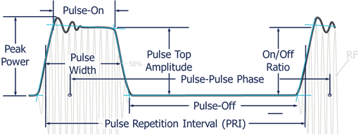
RF pulse characteristics such as those illustrated below reveal a great deal about a radar's capability. Electronic Warfare (EW) and ELectronic lNTelligence (ELINT) experts specialize in the study of these pulsed signals. Pulse characteristics provide valuable information about the type of radar producing a signal and what its source might be - sailboat, battleship, passenger plane, bomber, missile, etc.

Pulsed radar typically uses very low duty cycle RF pulses (< 10%). Range and resolution are determined by the pulse repetition frequency (PRF), pulse width (PW), and transmit power. A wide PW generally provides better range, but poor resolution. Conversely, a narrow PW has less range, but better resolution. This relationship constitutes one of the fundamental trade-offs in radar engineering. Pulse compression with a modulated carrier is often used to enhance resolution while maintaining a narrow PW allowing for higher power and longer range.
The Pulse Repetition Interval (PRI) is the time the pulse cycle takes before repeating. It is equal to the reciprocal of the PRF or Pulse Repetition Rate (PRR), the number of transmitted pulses per second. PRI is important because it determines the maximum unambiguous range or distance of the radar. In fact, pulse-off time may actually be a better indication of the radar system's maximum design range.
Traditional radar systems employ a transmit/receive (T/R) switch to allow the transmitter and receiver to share a single antenna. The transmitter and receiver take turns using the antenna. The transmitter sends out pulses and during the off-time, the receiver listens for the return echo. The pulse-off time is the period the receiver can listen for the reflected echo. The longer the off-time, the further away the target can be without the return delay putting the received pulse after the next transmitted pulse. This would incorrectly make the target appear to be reflected from a nearby object. To avoid this ambiguity, most radars simply use a pulse-off time that is long enough to make echo returns from very distant objects so weak in power, they are unlikely to be erroneously detected in the subsequent pulse's off-time.
The figure below illustrates the need for pulse compression to obtain good range and resolution. Wider PWs have higher average power, which increases range capability. However, wide PWs may cause echoes from closely spaced targets to overlap or run together in the receiver, appearing as a single target. Modulated pulses mitigate these issues, providing higher power and finer resolution to separate closely spaced targets.

Pulse power
Another consideration for the maximum range of a radar is the transmitted power. Peak power is a measure of the maximum instantaneous power level in the pulse. Power droop, pulse top amplitude, and overshoot are also of interest.
Pulse top amplitude (Power) and Pulse Width (PW) are important for calculating the total energy in a given pulse (Power x Time). Knowing the duty cycle and the power of a given pulse, the average RF power transmitted can be calculated (Pulse Power x Duty Cycle).
Radar equation
The Radar Equation defines many of the engineering trade-offs encountered by radar designers.

The radar equation relates the expected receive power (Pr) to the transmitted pulse power (Pt); based on transmit antenna gain (Gt), area of the receive antenna (Ar), target cross section (aka reflectivity) σ, range from the transmitter antenna to the target (Rt), and range of the target to the receive antenna (Rr).
Unlike many communications systems, radar systems suffer from very large signal path losses. The round-trip distance is twice that of a typical communications link and there are losses associated with the radar cross-section and reflectivity of targets. As you can see from the Radar Equation, the range term is raised to the fourth power in the denominator, underscoring the tremendous signal power losses radar signals experience.
Using the radar equation, the received signal level can be calculated to determine if sufficient power exists to detect a reflected radar pulse. Combining multiple pulses to accumulate greater signal power and average out the noise is also helpful for increasing the detection range.
Pulse width is an important property of radar signals. The wider a pulse, the greater the energy contained in the pulse for a given amplitude. The greater the transmitted pulse power, the greater the reception range capability of the radar.
Greater pulse width also increases the average transmitted power. This makes the radar transmitter work harder. The difference in decibels between the pulse power and average power level is easily calculated using ten times the log of the pulse width divided by the pulse repetition interval.
Range is therefore limited by the pulse characteristics and propagation losses. The PRI and duty cycle set the maximum allowed time for a return echo, while the power or energy transmitted must overcome the background noise to be detected by the receiver.
Pulse width also affects a radar’s minimum resolution. Echoes from long pulses can overlap in time, making it impossible to determine the nature of the target or targets. A long pulse return may be caused by a single large target, possibly an airliner, or multiple smaller targets closely spaced, possibly a tight formation of fighter aircraft. Without sufficient resolution, it is impossible to determine the number of objects that actually make up the echo return. Narrow pulse widths mitigate the overlapping of echoes and improve resolution at the expense of transmit power.
As such, pulse width affects two very important radar system capabilities -- resolution and detection range. These two qualities trade off against each other. Wider pulse longer-range radars offer less resolution, whereas narrow pulse shorter range radar have finer resolution.
Narrow pulses also require greater bandwidth to correctly transmit and receive. This makes the pulse's spectral nature also of interest, which must be considered in the overall system design as you can see in the illustration below.

While unmodulated pulsed radars are relatively simple to implement, they have drawbacks including relatively poor range resolution. To make the more efficient use of transmit power and optimize range resolution, radars modulate pulses using the following modulation techniques:
- Linear FM chirps -- The simplest and most common pulse modulation scheme is the linear FM (LFM) chirp. Sweeping the carrier frequency throughout a pulse results in every part of a pulse being distinct and discernable. This enables pulse compression techniques in the receiver to improve range resolution and transmit power efficiency.
- Phase modulation -- Phase modulation can also be used to differentiate segments of a pulse and is often implemented as a version of Binary Phase-Shift Keying (BPSK). There are specific phase coding schemes, such as Barker Codes, to ensure orthogonality of the coding and range resolution.
- Frequency hopping – This approach involves several frequency hops within a pulse. When each frequency has a corresponding filter with the appropriate delay in the receiver, all segments can be compressed together in the receiver. If the frequency hopping sequence remains the same for all pulses, then the receiver compression can even be implemented with a simple Surface Acoustic Wave (SAW) filter. The variable frequency pattern used by hopping pulses can reduce susceptibility to spoofing and jamming and help with interference problems.
- Digital modulation -- Digital signal processing enables more complex pulse modulations. For example, more effective anti-spoofing can be accomplished using M-ary PSK or QAM modulations that resemble noise rather than coherent frequencies to make detection more difficult. Other information can be encoded into digital modulations as well.
Basic pulsed radar using time-of-flight to measure target range has limitations. For a given pulse width, the range resolution is limited to the distance over which the pulse travels. When multiple targets are at nearly equal distance from the radar, the return from the farthest target will overlap the return from the first target. In this situation, the two targets can no longer be resolved from each other with just simple pulses.
Using a short pulse width is one way to improve distance resolution. However, shorter pulses contain proportionately less energy, preventing reception at greater range due to propagation losses. Increasing the transmit power is often impractical, such as for aircraft radar due to power constraints.
The answer to these challenges is pulse compression. If a pulse can be effectively compressed in time, then the returns will no longer overlap. Pulse compression allows low amplitude returns to be “pulled” out of the noise floor. It is achieved by modulating the pulse in the transmitter so different parts of the pulse become more discernable. The actual time compression is accomplished by the radar receiver.
The most common pulse compression technique is linear frequency modulation (LFM). An LFM pulse or chirp is one where the pulse begins at one carrier frequency, then ramps linearly, up or down to an end frequency. Compression is achieved in the receiver by passing the signal through a matched filter as shown below. This filter is designed to have a delay characteristic matched to the LFM frequency range, and delays portions of the modulated signal proportional to the carrier frequency.

When a pulse entering the receiver is a target return, there will likely be multiple close reflections due to the different surfaces of the target. If the compression signal processor has sufficient resolution, it can separate each of these reflections into discrete narrow pulses.
Another common pulse compression technique employs binary phase shift keying, or BPSK modulation, using a Barker coded sequence as shown below. Barker codes are unique binary patterns that auto correlate against themselves at only one point in time. Barker Codes can vary in length from 2 - 13 bits, providing a corresponding compression ratio of 2 - 13. The compression is achieved in the receiver by sensing the auto-correlation of the Barker sequence within the detected pulse.

Now that you have a basic understanding of radar signals, it’s time to move on to measuring them. In the next installment we’ll look at the lifecycle of radar measurement tasks, which can vary significantly depending on the job to be done and type of radar you are characterizing. In the meantime, be sure to check out our radar and electronic warfare application site.